Linking MS Excel to Evernote

Okay, if you don’t use or know what Evernote is, have a look at https://evernote.com/ and also check it out on https://www.youtube.com/

Basically, as the name suggests it is a note taking application which runs on all major platforms. There is a free version, that will do most people and then further paid versions with more options to satisfy Premium and business Users.

On a personal note (excuse the pun), I am a big fan of Evernote, and been using it since March 2009. The trick to get the best out of Evernote, is to add everything to it, the more it is used the better it becomes.

So, back to business. Obviously Microsoft Excel is awesome :-) however, it may not be the best way to record / store or manipulate data, but its ease of use and global popularity makes it a strong contender for certain tasks.

So you have created a spreadsheet and recorded loads of data (say research from various sources). You have even linked the cells to the URL which contains the original data..  All very good, but what happens if that link becomes dead??

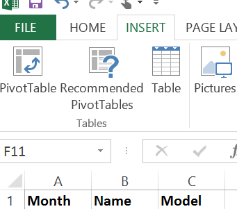
Note: Just as a quick pointer to insert a hyperlink press Ctrl & K, or go to the Insert Tab and select Hyperlink as shown below..

You will then be presented with “Insert Hyperlink” and asked to insert your Address, i.e. the URL of that you have just researched.

  

One of Evernotes main strengths is to collect data from all sorts of sources then store, retrieve and present them in a very searchable and usable way. So it makes sense that you link to your Evernote stored Note that you may have annotated etc.

To do this Right Click on the Note thumbnail as shown below..

You will then be presented with the following menu.  Select Share and Copy Note URL to Clipboard.

Now go back to your Insert Hyperlink as discussed earlier and Paste the URL and Click on OK.

Now when you click on that cell, you will be taken to a read only version of the Note, giving you much more in-depth information.

Please Note: Microsoft OneNote is also pretty awesome and is totally free, the same principles can be applied. It is definitely worth a look, if you are not aware of it. I personally use both for different reasons.

Thanks for taking the time to read this blog, I hope it may be of some use to someone :)

www.briancunningham.co.uk
keep learning

Bing Maps in Excel

Just a very quick and fun feature in Excel 365 (or 2013) is the ability to add a Bing Map and plot locations from a data set in your spreadsheet.

To try this open a new Excel spreadsheet, click on the Insert tab and then select Bing Maps under the Apps section.

This will insert a new Bing Map in the center of your table, it will also offer to insert sample data for you. 

We will close the window offering the sample data and then move and re-size the map.

To move the map, click on its edge, where you will see the cross arrows, now just click and drag.
To re-size, again click on its edge, but this time use the drag handles to re-size the map.
You can also zoom in and out or drag the the map to your desired location.


So now you have your map to the correct size and moved to where you want it, lets enter some data. 
Use a header, lets use Places, then enter a list of the places where you want pins to be placed on the map.

Now highlight the cells that contain the header and the place names. You are best to highlight more cells in the column if you are going to add more place names to be plotted.
This is column J in this example.

Once highlighted, click on the pin icon at the top of the map app, as shown below.

The map will automatically plot and zoom into the plotted area as such.

Very quick and simple, it will even does postcodes and countries also, try it.

Also try adding the Place header and one location, now highlight the cells that will contain the place names (or postcodes). Now each time you add a location the map will zoom in or out appropriately to include the new place name.


Now, say I really wanted to plot Coleraine as Coleraine USA, not Northern Ireland, then just put a comma after Coleraine and add USA ( Coleraine, USA )
If in doubt, do add the country as well as the town / city. 
The map will re-plot and zoom to cover all plotted locations.

Not all that useful on its own, but add a data set, say that contains sales figures, locations, etc. Also add a graph from this data set, this will very quickly enhance any presentation without much effort.
As always, the best way to learn and discover more is to play about with it, enjoy.

www.briancunningham.co.uk
keep learning

Basic PivotTable

PivotTables a probably one of the best features of Microsoft Excel, most people have not bothered too much with them as they think they might be very complicated or not that useful. 

In this blog, I hope to show you just how easy they really are and hope that my example will give you some inspiration on what you can use PivotTables for. 

I am going to use a scenario of a boat sales yard, it has 3 sales people and 3 types of boats that they sell. 
Not very imaginative, I know but this will keep it simple and give you a good grasp of the power of PivotTables. The data set consists only of the columns containing the Month the sale was made, the sales persons Name and the Model of boat sold:

So we can see we have 31 sales in a 3 month period. The data has just been recorded but is not really much use in this format. But with a couple of clicks on the mouse, it will be a lot more presentable and understandable.

First we will open the worksheet that contains the data set of the sales. 
Now open the Insert Tab at the top, and select the PivotTable icon

The Create PivotTable input box will appear. If the Table Range (highlighted below) is empty, just click in the text box and select the range you require, including the headers and select OK.
I have selected for the PivotTable to be created in a new Worksheet.

A new sheet will now appear with the following, do not be put off by what you see, it really is very simple, I will explain.
We will concentrate on the image to the right (PivotTable Fields), the image on the left is where the results will be displayed.

            

As you can see, Month, Name and Model are displayed in the PivotTable Fields area and below that are four sections called Filters, Columns, Rows and Values.

So, remember we had 31 rows of data that really did not make a lot of sense. This really is how useful and easy PivotTables are.
Just drag the Name (as highlighted in green above) into the Rows section as below, repeat for Month and Drag the Model into the Values section.

And this is what the PivotTable returns for you:
Here we can see the total sales figures broke down by the sales person and further by the month.

By simply moving the Month above Name in the Rows section, you will get it broke down by the Months first, then the sales person.

This happens immediately without having to do any further formatting or input.

Say we wanted the data displayed like this:

Then just set the order as putting the Month in Columns, Name in Rows and Model in Values:

Now by simply dragging the Model into the Rows the result will be broke down by the type of boat sold by each person for each month, giving a more detailed, useful and understandable data set.

Drag the Model above Name to group by the Model rather than the Name and the data set will be displayed as such:

So there you have it, I hope you will agree that PivotTables are really simple and will be very useful for displaying data in a more meaning and presentable manner.
PivotTables are the gem in Excels crown.

As always, this was a very basic tutorial, and the best way to learn and discover more is to play about with it, enjoy.


Note, I used Microsoft Excel 365 in this example, but the Pivot Table has existed in MS Excel since 2003 (at least) 

www.briancunningham.co.uk
keep learning

VLOOKUP - Auto populate cells based on a value of another cell

Searches for a value in the first column of a table array and returns a value in the same row from another column in the table array - As explained by Microsoft..

Okay in this example, I am going to use employee details and again, keep it very simple..
We have a spreadsheet with the employee details as shown below:

In another sheet or even spreadsheet, we want to get the phone number for one of the employees based only on their Employee ID number....
There are a few simple steps to this:

• First off, create a list based on EmpID as seen in the Blog - Drop Down List

• Now click on the cell you want to be auto-populated (we are going to add the first name, last name and phone number, so this will be repeated in 3 cells).  If you have read this far, your probably best using the formula wizard found under Look Up & Reference in the Formulas Tab as below (Excel 2010).  

• A window will appear asking you input the arguments for the function as below

A quick explanation of this window:

• The Lookup_value is the cell containing the list..  We are using EmpID, click in the text box and then click on the cell containing the list.
• Table_array, this is the area of the sheet that contains the info you want returned..  Again, click on the text box and then highlight the cells containing the required info, first name, last name and phone number..  Don't worry if you have to include other cells, in our example we have to include StartDate and Dept..
• Col_index_num, this is the index of the column that will return the requested data.  Our example has last name, then first name in the original data set, but we want to show the first name followed by the last name, then the phone number, so enter 3 here for the third column which contains the first name. 
• Range_Lookup, this is a logical - True or False argument, where False equals that you want an exact match returned and True means that you want the closest match returned..

Now follow the above steps for the last name and phone number in your desired cells, most probably next to the first name..

Before you use the formula wizard for all three, read below, it is faster either writing the formula or copy and paste, you will only need to adjust the Col_index_num for last name and phone number..

Remember last name was first in the original data set, so we used 3 as the column index for first name, now use 2 as the column index for the last name, and you have changed the order of the way the name is displayed..

The Formula

If you are like me, and would rather input the formula here it is:

=VLOOKUP(B3,Sheet1!A2:F5,3,FALSE)

Note the 4 arguments: 

Lookup_value = B3

Table_array = Sheet1!A2:F5    (the data set is on Sheet1 and is held in cells A2 to F5)

Col_index_num = 3    (this is the first name column)

Range_Lookup = False  (we want an exact match)

There is also hlookup, used for rows...

For Aries 

www.briancunningham.co.uk
keep learning