Bing Maps in Excel

Just a very quick and fun feature in Excel 365 (or 2013) is the ability to add a Bing Map and plot locations from a data set in your spreadsheet.

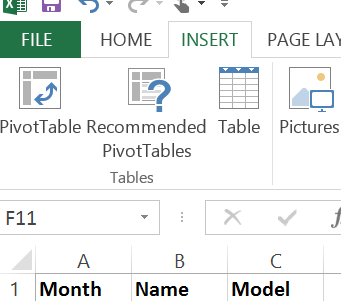
To try this open a new Excel spreadsheet, click on the Insert tab and then select Bing Maps under the Apps section.

This will insert a new Bing Map in the center of your table, it will also offer to insert sample data for you. 

We will close the window offering the sample data and then move and re-size the map.

To move the map, click on its edge, where you will see the cross arrows, now just click and drag.
To re-size, again click on its edge, but this time use the drag handles to re-size the map.
You can also zoom in and out or drag the the map to your desired location.


So now you have your map to the correct size and moved to where you want it, lets enter some data. 
Use a header, lets use Places, then enter a list of the places where you want pins to be placed on the map.

Now highlight the cells that contain the header and the place names. You are best to highlight more cells in the column if you are going to add more place names to be plotted.
This is column J in this example.

Once highlighted, click on the pin icon at the top of the map app, as shown below.

The map will automatically plot and zoom into the plotted area as such.

Very quick and simple, it will even does postcodes and countries also, try it.

Also try adding the Place header and one location, now highlight the cells that will contain the place names (or postcodes). Now each time you add a location the map will zoom in or out appropriately to include the new place name.


Now, say I really wanted to plot Coleraine as Coleraine USA, not Northern Ireland, then just put a comma after Coleraine and add USA ( Coleraine, USA )
If in doubt, do add the country as well as the town / city. 
The map will re-plot and zoom to cover all plotted locations.

Not all that useful on its own, but add a data set, say that contains sales figures, locations, etc. Also add a graph from this data set, this will very quickly enhance any presentation without much effort.
As always, the best way to learn and discover more is to play about with it, enjoy.

www.briancunningham.co.uk
keep learning

Basic PivotTable

PivotTables a probably one of the best features of Microsoft Excel, most people have not bothered too much with them as they think they might be very complicated or not that useful. 

In this blog, I hope to show you just how easy they really are and hope that my example will give you some inspiration on what you can use PivotTables for. 

I am going to use a scenario of a boat sales yard, it has 3 sales people and 3 types of boats that they sell. 
Not very imaginative, I know but this will keep it simple and give you a good grasp of the power of PivotTables. The data set consists only of the columns containing the Month the sale was made, the sales persons Name and the Model of boat sold:

So we can see we have 31 sales in a 3 month period. The data has just been recorded but is not really much use in this format. But with a couple of clicks on the mouse, it will be a lot more presentable and understandable.

First we will open the worksheet that contains the data set of the sales. 
Now open the Insert Tab at the top, and select the PivotTable icon

The Create PivotTable input box will appear. If the Table Range (highlighted below) is empty, just click in the text box and select the range you require, including the headers and select OK.
I have selected for the PivotTable to be created in a new Worksheet.

A new sheet will now appear with the following, do not be put off by what you see, it really is very simple, I will explain.
We will concentrate on the image to the right (PivotTable Fields), the image on the left is where the results will be displayed.

            

As you can see, Month, Name and Model are displayed in the PivotTable Fields area and below that are four sections called Filters, Columns, Rows and Values.

So, remember we had 31 rows of data that really did not make a lot of sense. This really is how useful and easy PivotTables are.
Just drag the Name (as highlighted in green above) into the Rows section as below, repeat for Month and Drag the Model into the Values section.

And this is what the PivotTable returns for you:
Here we can see the total sales figures broke down by the sales person and further by the month.

By simply moving the Month above Name in the Rows section, you will get it broke down by the Months first, then the sales person.

This happens immediately without having to do any further formatting or input.

Say we wanted the data displayed like this:

Then just set the order as putting the Month in Columns, Name in Rows and Model in Values:

Now by simply dragging the Model into the Rows the result will be broke down by the type of boat sold by each person for each month, giving a more detailed, useful and understandable data set.

Drag the Model above Name to group by the Model rather than the Name and the data set will be displayed as such:

So there you have it, I hope you will agree that PivotTables are really simple and will be very useful for displaying data in a more meaning and presentable manner.
PivotTables are the gem in Excels crown.

As always, this was a very basic tutorial, and the best way to learn and discover more is to play about with it, enjoy.


Note, I used Microsoft Excel 365 in this example, but the Pivot Table has existed in MS Excel since 2003 (at least) 

www.briancunningham.co.uk
keep learning